History Bernhard Riemann (1826-1866) was a German mathematician who was credited with some of the most important developments in modern mathematics. One operation that bears his name is the Riemann Integral. What is an Integral? An integral is the mathematical term for the area associated with a function. There are different types of integrals, but the simplest type of integral is called the Riemann integral. The Reimann integral represents the area between the graph of a function and the x-axis. So, we will investigate some strategies for finding this area.

The Riemann integral in 2-dimensions is defined on a given interval of the x. With symbols, we write the integral of amath f(x) endamath over x from a to b as:

Methods and Strategies

We want to approximate the integral of a function using the area of familiar shapes. To do this we must first divide the interval into a Partition, which just means that we want to split up the distance between a and b into equally spaced subintervals.

Example 1: Approximate amath \int_0^10 x^2 dx endamath. That is, we need to find the area underneath the parabola amath y=x^2 endamath beween the x-axis and the graph which is the shaded region in the graph to the right. Step 1: First we will divide the interval [0,10] into the partition P={0,2,4,6,8,10}. This splits the x-axis into the sub-intervals [0,2],[2,4],[4,6],[6,8],[8,10] Step 2: Now we will calculate the value for amath f(x)=x^2 endamath for each of the interval points from step 1. amath f(0)=0 , f(2)=4 , f(4)=16 , f(6)=36 , f(8)=64 , f(10)=100

Step 3:We will now approximate the area in one of three ways:

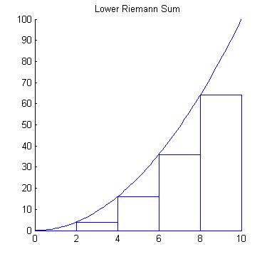
• Lower Reimann Sum
  

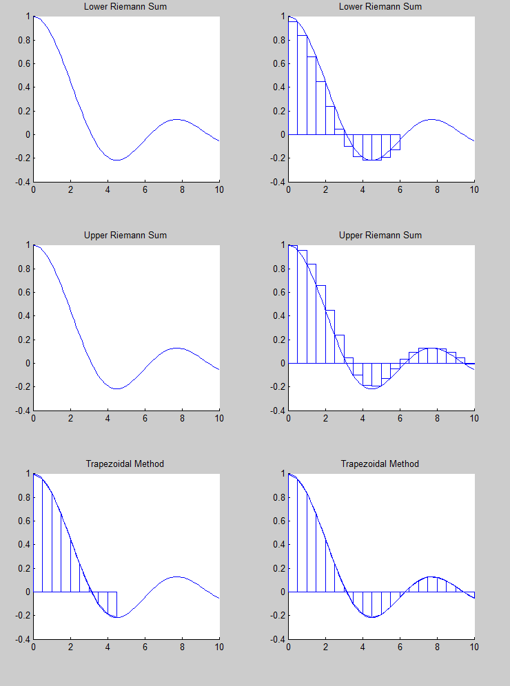
  For each subinterval amath [x_i,x_{i+1}] endamath, we will choose the smaller of the two values amath f(x_i) endamath or amath f(x_{i+1}). We will then draw the rectangle from amath x_i endamath to amath x_{i+1} endamath that has the height of the this smaller value. After we do this for each subinterval, we will have a plot like the one to the right. Now we will find the area of each rectangle and total the areas. amath \int_0^10 x^2 dx \approx 0 + 8 + 32 + 72 + 128 = 240 endamath As we can see from the gaps between the rectangles and the parabola, this is not a very good estimate.

  
  
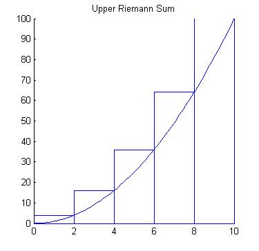
• Upper Riemann Sum
  

  For an upper Riemann Sum, we will consider each interval amath [x_i,x_{i+1}] endamath, but this time we will make our rectangles the height of the largest of the two values amath f(x_i) endamath or amath f(x_{i+1}) endamath. We will draw the rectangles as we did for the Lower Riemann Sum but we will use this larger height. We get the plot to the right for the Upper Riemann Sum. We can now find the area of the rectangles and total them to approximate the integral. amath \int_0^10 x^2 dx \approx 8 + 32 + 72 + 128 + 200= 440 endamath This is quite different than the Lower Riemann Sum approximation. Again, we can see from the plot to the right that we have a lot of extra space where the rectangles are above the parabola.

  
  
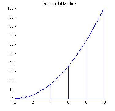
• Trapezoidal Method
  

  Using the rectangles above give us two very different answers (240 and 440). So, let's try a different geometrical shape that might fit the curve better ... a trapezoid. Recall that the formula for the area of a trapezoid with height h and bases b1 and b2 is amath $Area=\frac{1}{2}(b_1+b_2)h$ endamath So, we can use the values of amath f(x_i) endamath and amath f(x_{i+1}) endamath as the values of b1 and b2, and the height of the trapezoid is h=xi+1 - xi. We get the graph to the right and we can calculate the area of the trapezoids using the values of each amath f(x) endamath .

  amath \int_0^10 x^2 dx \approx 1/2(0+4)2+1/2(4+16)2+1/2(16+36)2+1/2(36+64)2+1/2(64+100)2=340 endamath
  As we can see from the graph, the trapezoids are a much better fit of the area under the curve.

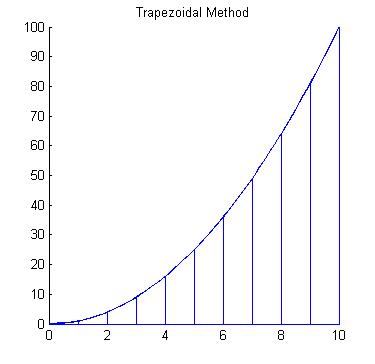
Try It: Now it is your turn. Use the trapezoid method to approximate the value of amath \int_0^10 x^2 dx endamath using a partition of 10 subintervals. In other words, we will divide the interval [0,10] into the partition P={0,1,2,3,4,5,6,7,8,9,10}. When we plot the trapezoids, we will get the graph to the right. Now download the RiemannSums.m file and open it up in Matlab. Use this program to test your approximation for this integral.

Programming Exploration

Let's use MatLab to explore these methods for finding an approximation for an integral. Use the RiemannSums.m to approximate the following integrals to within an error of 10^-3 by refining the number of intervals until the error is small enough.

• amath \int_0^10 sin(x) dx endamath
• amath \int_{-3}^3 x^3-5x^2+2 dx endamath
• amath \int_1^5 (2 sin(x))/x dx endamath

Related Links

• Riemann History from Johanneum Lüneburg School (Where Riemann attended)
• History of Riemann Integral from Dr. Allen, T.A.M.U.